Tutorial

Welcome to the Membrainy tutorial. This tutorial should guide you through the basic usage of Membrainy, as well as analysing some test systems and understanding the output graphs. Firstly, you will need to download the tutorial files here (171Mb).

This folder should contain the files:

• complex-membrane.gro
• electroporation_charmm.xtc
• electroporation_charmm.tpr
• library.mbr
• mixing_martini.xtc
• mixing_martini.gro
• pope-popg_gromos.trr
• pope-popg_gromos.gro

A few things to note beforehand: Please use the latest version of Membrainy. Membrainy assumes that you have GROMACS currently installed and located within your classpath. It also assumes that your GROMACS binaries have typical names (e.g. "editconf" and "g_potential"). If you used a suffix for all gromacs binaries (e.g. editconf_mpi) then please add the argument "-g_suffix _mpi" with every step in this tutorial, replacing "_mpi" with your chosen suffix. You will also need to have the software "xmgrace" installed on your system in order to view the output plots. This is not required to run the analysis however. Xmgrace can be obtained here.

Tutorial 1: Mixing entropy (Martini)

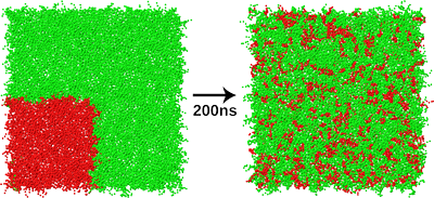
The ability to quantify a mixing/demixing entropy in mixed lipid systems is implemented into Membrainy. This technique was established by Brandani et al. in this paper. In the tutorial files, you should find two files: mixing_martini.xtc and mixing_martini.gro. These files contain a system that was initialised such that one quadrant of the bilayer is entirely POPC lipids (shown in red) with the rest of the bilayer containing POPE lipids (green). You could describe this as a perfectly demixed system. It is known that these lipid types mix well, so we are expecting the system to mix over time. The provided xtc contains a 200ns trajectory with sampling every 1ns. We can analyse this system as follows: Which will begin analysing the xtc. It is worth noting that the default force field in Membrainy is set to CHARMM, so if you forget to type "-ff martini", Membrainy will detect something isn't quite right and terminate. It also doesn't matter what you use for the "-s" input, it could be a gro file from any point in time, or the tpr file - Membrainy uses this file to generate the topology of the system, which isn't included in the xtc file. If all goes smoothly, you should receive the following output: Membrainy has analysed the .gro file and determined the system contains two lipid types: POPC and POPE. It has also identified the reference atoms, with atom type PO4. 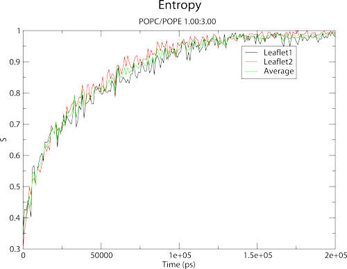Two files should now exist in your current working directory: entropy.agr, and entropy_scaled.agr. For each frame, Membrainy is looking to see which lipids are neighboured to each other. It does this by identifying a reference atom, usually the phosphorous atom, and calculating a distance vector between each reference atom to determine the closest lipid. This information is then binned into a probability matrix and normalised. The entropy is output over time into entropy.agr, and a scaled entropy is calculated such that the theoretical maximum entropy is always 1. Finally, we can view the entropy plot by running: which should yield the following: The graph shows the entropy for each leaflet, and also provides an average for both leaflets. You should note that Membrainy has atomatically assigned axis labels, plot legends and a title/subtitle for your convenience.

Tutorial 2: Electroporation of a POPC double bilayer (CHARMM)

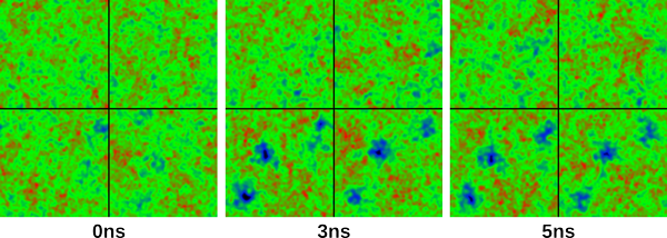
Among the implemented tools within Membrainy is the ability to scan the voltage against time for double bilayer systems and to produce 2D surface maps. This voltage normally fluctuates in NPT ensembles, and will change dramatically in systems undergoing electroporation. The two files provided: electroporation_charmm.xtc and electroporation_charmm.tpr contain a 5ns trajectory of a POPC double bilayer with an ion imbalance of +50. This achieves an initial voltage of around -4V, which immediately establishes 3 large pores in one of the bilayers. Membrainy can visualise the pore formation through the surface maps tool, and also look at the voltage against time. However, let's begin by looking at the surface maps. These maps are produced by binning the heights of all atoms in each leaflet, and applying a Gauss-Seidel algorithm to the bins. Run Membrainy as follows: This will load the graphical interface for the surface maps, and begin scanning the trajectory. Each frame should be loaded sequentially and updated on the screen, with each leaflet represented on the interface. The numbers at the top left represent the leaflet number (for double bilayers we have 4 leaflets). The leaflets are numbered from the bottom of the system box to the top, so leaflets 1 and 2 indicate the lower bilayer, while 3 and 4 indicate the upper bilayer. Once all 50 frames are loaded, move the frame slider (located at the bottom left, next to the "Frame: 50/50") back to the 0/50 position, and hit capture. You should see an output on the terminal saying: which has written the surface map to a png file, and placed in the folder "images" in the current working directory. Do the same for 30/50 and 50/50, and you should have three images identical to the following: which show surface snapshots taken at 0ns, 3ns and 5ns. In 3ns and 5ns, you can easily see three pores being established in leaflets 3 and 4. Cool, huh? You may also want to play around with the positioning of the pores before capturing an image. You can click and hold the mouse button anywhere on the surface map display, and drag the mouse around. This is handy if there is a particular part of the membrane you wish to centre before capturing an image. Be sure to play around with the "Mirror images" and "Show Ions" options. The slider to the right of the Show Ions box allows you to set the distance (from the centre of the bilayers) of which ions you wish to view. Setting this to around 25 will only show ions within 25 Angstroms of the bilayer centre. At the moment you cannot distinguish between cations and anions, but this will likely come in a future update. You may also notice that some sliders are greyed out. These will become available when loading a single gro file as an input, and will allow you to tweak the resolution, number of iterations of the Gauss-Seidel algorithm, and the intensity of the peaks on the surface maps.

Next we will look at the voltage against time plot. Run the following: As default, Membrainy will set the -dt option to 500ps and -sl to 1000 slices. The dt option is needed as the trajectory must be divided into small time windows in order to calculate an electrostatic potential for each window. The voltage is then extrapolated from the potential, taking the average potential from the central water compartment between the two bilayers. The -sl option is identical to that used in g_potential, which divides the box into "slices" to calculate the electrostatic potential per slice.

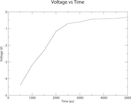
You should have the following output: Membrainy has automatically created an index.ndx file, although if you already had one in the current working directory, it would be detected and used. Membrainy then executes g_potential in 500ps windows, which should output the file potential_0-500.xvg. Membrainy then detects the middle of the box to be 10.15nm, and uses this as a reference to scan the central compartment. The potential between the two bilayers is then averaged to produce a voltage, which is -4.4V. This voltage was averaged from 255 points taken from potential_0-500.xvg, between 7.55nm and 12.71nm, which is where one bilayer ends and the other begins. Finally, there should be the file voltage_vs_time.agr within your current working directory, which looks like this: The plot shows a dramatic drop in voltage over the first 2-3ns, which is achieved through both electrostriction and ions travelling through the pores to neutralise the ion imbalance.

Tutorial 3: A standard membrane trajectory (GROMOS)

Membrainy can analyse the standard properties of membranes: area per lipid, bilayer and leaflet thickness, deuterium order parameters, gel percentage and headgroup orientations. We will use the provided pope-popg-gromos.trr and pope-popg-gromos.gro files, which contain 50ns of a POPE/POPG (3:1) double bilayer with sampling every 1ns (to minimise the file size, normally the sampling would be much more frequent). Run the following: which will begin the analysis. If you have a second terminal window open, you can monitor the output files as the analysis is being run as these are produced every frame. You should note that trr files are a little slower to read as they contain three times as much data as xtc files. Membrainy discards the forces/velocities, so you will notice a substantial speed increase if you only use xtcs. Once the analysis is complete there should be several new files in your working directory.

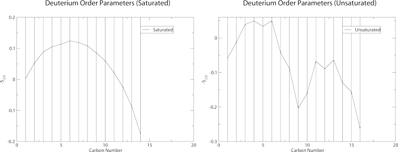
First, lets take a look at the order parameters. Membrainy calculates order parameters based on the formula described in this paper. You will see the files POPE1.agr, POPE2.agr, LPOPG1.agr, LPOPG2.agr, saturated-order-parameters.agr and unsaturated-order-parameters.agr. For the most part, you will only need the latter two files, which contain a total average of all order parameters across all leaflets in the system. If this was a double bilayer system there would be additional files called saturated-compartments.agr and unsaturated-compartments.agr, which would contain an average of leaflets 1 + 4 and 2 + 3 (or the inner and outer leaflets in the system). The additional files, e.g. POPE1.agr contain the individual order parameters for each acyl chain in each leaflet. Typing the following: and Should yield these graphs: which also contain the standard deviation in the order parameters. These plots will not be particularly accurate as the sampling in the trr file is very low. Order parameter plots work best with a sampling of around 10-20ps.

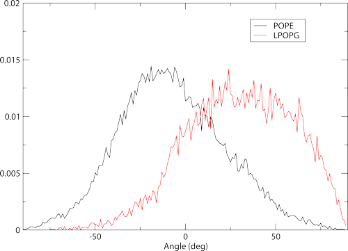
Headgroup orientations are calculated using two reference atoms on the lipid head. Membrainy will automatically detect which atoms to use, one typically being the phosphorous and the other being the last polar atom on the headgroup. There are two files produced here, headgroup-angles.agr and headgroup-angles-leaflets.agr. For most scenarios we only need to focus on the first file. Load it with xmgrace to see the plot: which shows histograms containing the distribution of headgroup orientations. These also work best with 10-20ps samples to produce a smoother distribution. It is worth noting that in higher sampling examples, you will begin to see a defect in the plots around 0 degrees. This is not a bug - This is due to the precision error in the xtc, which rounds certain orientations to specific bins. A workaround will be provided in a future update.

Finally, you should also see output graphs for leaflet and membrane thickness, area per lipid and gel percentage over 50ns. These are fairly straightforward to interpret.

Tutorial 4: Using an external library file for non-standard membrane systems

Membrainy contains an in-built library of common lipids, residues, force fields, cholesterols, ions etc., meaning that for many standard membrane systems, it will "just work". However for non-standard membrane systems, Membrainy is capable of importing an external library file, allowing the user to specify custom lipids, residues, force fields etc., that are not included in the in-built library. The external library file can also be used to override the internal library for cases where non standard naming conventions are used.

In this example, we will modify an external library file so that Membrainy can recognise and analyse a highly diverse and complex membrane system, taken from a 'realistic' membrane found in this paper. The provided complex-membrane.gro file contains a mixture of standard lipids and two non-standard lipids DLiPC and DLiPE, as well as two cholesterols STIG and SITO. Firstly, run Membrainy with the gro file as normal: Which will yield: Although this looks normal, Membrainy has ignored all entries of STIG, SITO, DLIPC and DLIPE in the gro file, and would fail to perform an analysis on these molecules. Open library.mbr in any text editor. Inside this file we will see a template containing various flags such as [ FF ], [ Residue ], [ Water ] etc. We can use these flags to augment the in-built library with new information. Firstly we want to add values under the [ Cholesterol ] flag to include the new cholesterol names: Secondly, we want to add values under the [ Lipid ] flag to include the missing lipids We can now rerun Membrainy and attach the external library file: You will see that Membrainy is now recognizing the new lipids and cholesterols, and has correctly identified 512 lipids in the bilayer.

Before we can perform an analysis, we need to provide Membrainy with a little more information regarding the naming conventions and structure of the headgroups and tails. We can do this by using the [ LipidHead ] and [ LipidTail ] flags. It is worth noting that these flags are optional and are only required if you plan on using one of the analytical techniques that require this information, i.e. order parameters require information about the lipid tails but do not need headgroup information, whereas headgroup orientations do not need lipid tail information.

If we focus on DLIPC, we know that this lipid can be separated into DLI tails and a PC headgroup. Because the PC headgroup is already included in the in-built library, we do not need an entry for this. We do however need an entry for the DLI tails. Ammend the library file to contain the following: In this entry, we set the 'Name' flag as DLI so that Membrainy can identify that both DLIPC and DLIPE will contain DLI tails. We set 'FF' to CHARMM because we are using the CHAMM force field (and naming convention) for our system. Finally, we need to list all of the carbon atoms in each tail travelling down the tail, ensuring that the first and last carbons are included (but not including the carbon that connects both tails together). If our lipid tail is unsaturated, we also need to include the four carbons involved in the double bond, i.e. C-C=C-C. For tails with multiple double bonds, list each group of four carbons back to back, noting that sometimes the same carbon may be listed twice if belonging to two double bond groups. The resulting line should always contain a multiple of four carbons. If the tail is saturated, leave the entry blank.

The CHARMM naming convention sometimes uses a unique number or letter as a suffix on the hydrogens attached to unsaturated carbons. This can easily be seen when looking at POPC lipids, in which the CHARMM naming convention appears different to other lipids. If your lipid uses this naming convention, you can add this suffix using the 'UnsatSuffix' flag, as shown in the PO example entry in the library file.

As an example of the [ LipidHead ] flag, see the PE entry in the library file. Similarly to the tail, we use the 'Name' flag to identify the headgroup name, where PE can be used for any lipids containing a PE headgroup (POPE, DLPE, etc.). The 'HeadgroupAtoms' flag allows us to list the atoms located in the headgroup, which is primarily used by the shells code when calculating distances between proteins and lipid headgroup atoms. Lastly, the 'ReferenceAtoms' flag allows us to list the two reference atoms we wish to use for headgroup orientation calculations.

Going back to our membrane system, we can now instruct Membrainy to perform an order parameters analysis and a headgroup angles analysis: Which should run successfully and produce analysis outputs containing each lipid.